From BOL to EOL: Tracking Lifetime Drift in a Buck Converter with SIMBA
Power converters are usually validated at nominal conditions, with fresh components and room-temperature parameters. That is a necessary first step, but it is not enough. A design that looks comfortable at Beginning of Life (BOL) can move much closer to its limits at End of Life (EOL) once the passive components have drifted.
This article shows a simple and defensible way to start a BOL/EOL study in SIMBA. Instead of trying to model every aging mechanism at once, we focus on one parameter drift that is both common and visible in the waveforms: output-capacitor capacitance loss in a buck converter. The result is already instructive: the converter still regulates, but the output-voltage ripple changes strongly over lifetime.
1. Why BOL-only validation is not enough
In real hardware, lifetime drift does not usually appear as a spectacular failure on day one. It appears as a gradual reduction of design margin:
- output ripple increases,
- control effort changes,
- losses move,
- thermal headroom shrinks,
- compliance margins become less comfortable.
That is exactly why BOL/EOL studies matter. The engineering question is not only “does the converter work when the parts are new?” but rather “does it still meet the target when the parts have drifted?”
2. Case study used here
The study below is based on the official SIMBA Python design example simba.DesignExamples.BuckConverter() executed on 2026-09-17.
Model settings
| Parameter | Value |
|---|---|
| Topology | Buck converter |
| Input voltage | 50 V |
| Duty cycle | 0.5 |
| Switching frequency | 5 kHz |
| Inductor | 1 mH |
| Load | 5 Ω |
| Nominal output capacitor | 100 µF |
The switching frequency may look low by modern converter standards. It comes directly from the official SIMBA example and was intentionally kept unchanged here to preserve reproducibility.
Figure 1 shows the actual SIMBA schematic used as the basis of the study.

3. BOL / mid-life / EOL assumptions
For this first article, only the output capacitor is aged. This is intentionally narrow: it keeps the interpretation clean and makes the workflow easy to reproduce.
| Lifetime state | Output capacitor value |
|---|---|
| BOL | 100 µF |
| Mid-life | 70 µF |
| EOL | 40 µF |
The EOL point was intentionally selected as a severe degradation scenario corresponding to a 60% capacitance loss. It is not presented here as a universal aging law tied to one capacitor technology, one temperature, or one lifetime in hours. It is a practical parameter-drift scenario used to answer a concrete question: what happens to the converter waveforms and KPIs when the output capacitor loses a large part of its effective capacitance over lifetime?
In practice, ESR growth is often as important as capacitance loss in aged capacitors. It is intentionally excluded from this first workflow demonstration and should be added in a dedicated follow-up study.
4. What the transient simulations show
The three SIMBA transient runs keep the same operating point and only change the output-capacitor value.
BOL vs EOL waveform view
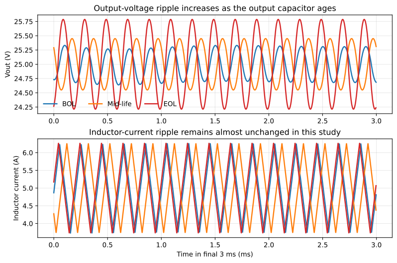
The main visible effect is on the output voltage. As the capacitor value decreases, the converter still regulates around 25 V, but the ripple envelope becomes much larger.
By contrast, the inductor-current ripple remains almost unchanged in this study. That is expected: we changed the output capacitor, not the switching frequency, duty cycle, or inductance.
5. First-order analytical validation
For an ideal buck converter in continuous conduction mode, a first-order estimate of the capacitive ripple is:
[ \Delta V \approx \frac{\Delta I_L}{8 f_s C} ]
This does not include ESR effects, non-ideal switching behavior, or detailed waveform distortion. But it is a useful baseline for checking whether the simulated trend remains physically coherent.
| Case | Theory (mVpp) | SIMBA (mVpp) | SIMBA / Theory |
|---|---|---|---|
| BOL | 626.6 | 665.0 | 1.061 |
| Mid-life | 894.6 | 901.4 | 1.008 |
| EOL | 1579.3 | 1573.4 | 0.996 |
The agreement is good enough for the intended purpose of the article: the simulated ripple follows the expected inverse relationship with capacitance, while keeping the full transient waveform available for deeper analysis.
6. KPI comparison
| Case | Capacitance | Vout avg | Vout ripple | Inductor ripple | Capacitor RMS current |
|---|---|---|---|---|---|
| BOL | 100 µF | 25.005 V | 665.0 mVpp | 2.507 App | 0.728 A |
| Mid-life | 70 µF | 25.005 V | 901.4 mVpp | 2.505 App | 0.723 A |
| EOL | 40 µF | 25.002 V | 1573.4 mVpp | 2.527 App | 0.731 A |
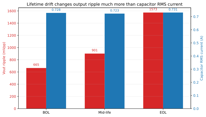
The message is straightforward:
- average output voltage barely moves,
- inductor ripple barely moves,
- but output-voltage ripple more than doubles from BOL to EOL.
In this specific study, the ripple rises from 665 mVpp at BOL to 1573.4 mVpp at EOL, i.e. a +136.6% increase.
7. Engineering interpretation
This is precisely why a BOL/EOL workflow is useful.
If an engineer looked only at the average output voltage, the conclusion would be that nothing important changed. But the transient waveforms say otherwise: the converter keeps the same nominal conversion ratio while its filtering performance degrades strongly.
That distinction matters in practice because many specifications are not written on the average value alone. They are written on:
- peak-to-peak ripple,
- downstream stress,
- EMI behavior,
- regulation margin under transients,
- allowable capacitor aging budget.
A simple compliance-style reading makes the point clearer:
- with a 2 Vpp ripple specification, all three cases remain compliant,
- with a 1 Vpp ripple specification, the EOL case fails while BOL and mid-life remain acceptable.
So even this simple one-parameter drift study already answers a real design question: is the initial capacitor choice still acceptable at EOL for the target ripple limit?
8. Why this is a good SIMBA workflow
The point of SIMBA here is not just to produce one more waveform plot. It is to make lifetime studies operational:
- keep one design,
- define BOL / mid-life / EOL parameter sets,
- run the same transient analysis automatically,
- compare waveform-derived KPIs,
- identify which specifications are the first to become fragile.
Once that workflow is in place, the next step is natural: instead of aging only the output capacitor, you can also introduce drift on:
- capacitor ESR,
- inductor DCR,
- MOSFET on-state resistance,
- magnetic parameters,
- thermal conditions.
That is where a true lifetime design-space exploration starts becoming valuable.
9. Limits of this first study
This article intentionally stays modest in scope.
- Only one aging mechanism is modeled here: capacitance loss.
- No ESR drift is introduced yet.
- No thermal feedback loop is included.
- The example is an official SIMBA buck example, not a product-specific industrial design.
So the result should be read for what it is: a clean first BOL/EOL workflow demonstration based on real SIMBA transient runs, not a complete lifetime qualification methodology.
10. Reproducing the study in SIMBA Python
The runs were executed with aesim.simba on 2026-09-17 from the official design example simba.DesignExamples.BuckConverter(). The only parameter changed between the three cases is the output capacitor value.
import os, sys
os.environ['DOTNET_SYSTEM_GLOBALIZATION_INVARIANT'] = '1'
os.environ['PYTHONNET_RUNTIME'] = 'coreclr'
sys.path.insert(0, '/fab/toolpacks/simba-python/site-packages')

import aesim.simba as simba
simba.License.Activate(os.environ['SIMBA_DEPLOYMENT_KEY'])

def run_case(c_value_farad):
    design = simba.DesignExamples.BuckConverter()
    for device in design.Circuit.Devices:
        if str(device.Name) == 'C2':
            device.Value = c_value_farad
    for device in design.Circuit.Devices:
        for scope in device.Scopes:
            scope.Enabled = True
    job = design.TransientAnalysis.NewJob()
    status = job.Run()
    return status, job
11. Conclusion
A BOL/EOL study does not need to start with a full aging physics model to be useful. A first parameter-drift exploration already helps answer a practical engineering question: which performance metrics are robust over lifetime, and which ones are not?
In this buck-converter example, average output voltage stays nearly unchanged from BOL to EOL, but output-voltage ripple increases sharply as the output capacitor ages. Under a loose ripple requirement the design may still pass at EOL; under a tighter one, the same converter can become non-compliant without any change in its nominal conversion ratio.
The important lesson is not that the converter stops working at EOL. It is that key specifications can be lost long before the converter stops regulating correctly. BOL/EOL analysis helps identify those hidden margin reductions early in the design process.
References
- R. W. Erickson, D. Maksimović, Fundamentals of Power Electronics, 2nd ed., Springer, 2001.
- SIMBA Documentation, Python Library and Design Examples,
doc.simba.io. - Application notes and datasheets on aluminum-electrolytic and polymer-capacitor aging mechanisms, ESR drift, and capacitance loss under temperature and ripple-current stress.
About the Author
Sophia is a power electronics engineer at Powersys, focused on SIMBA, JMAG, and practical simulation workflows for converter design, control, thermal behavior, and design-space exploration.
Transparency note — All numerical results reported in this article come from real transient simulations executed with SIMBA on 2026-09-17. In this first BOL/EOL example, the modeled lifetime drift is limited to output-capacitor capacitance reduction; no full electro-thermal aging loop is claimed here.


