Dead Time vs Current in a SiC Half-Bridge: A Practical SIMBA Exploration
A SIMBA-based exploration of how dead time and current interact in a SiC half-bridge, using the official double-pulse example and real transient simulations.
Abstract
Dead time in a SiC half-bridge is often entered once in the gate driver and then left untouched. In practice, it is a parameter that should be checked against the actual switching waveforms. In this study, I used the official SIMBA Double_Pulse_test example and ran real transient simulations while sweeping the inserted delay between the first turn-off and the second turn-on from 50 ns to 900 ns. On this specific operating point, the sweep does not reveal a spectacular switching-energy change. What it does reveal is a clean, reproducible workflow: longer dead time increases the interval spent at very low VDS before the second pulse, while the overlap power and the integrated turn-on metric decrease slightly. That makes this article less a claim of dramatic sensitivity and more a practical method: sweep dead time, inspect the real waveforms, and then decide whether the operating point is aggressive enough to justify a larger design-space exploration.
1. Why a practical workflow matters more than a fixed dead-time number
On a fast SiC stage, dead time affects at least three things at once:
- how long the switching node is allowed to settle before the next turn-on
- how much voltage-current overlap remains during the next commutation event
- how much margin is left before diode conduction or unwanted cross-conduction becomes a risk
That coupling is easy to talk about qualitatively and easy to oversimplify quantitatively. A fixed recommendation such as 100 ns or 200 ns is rarely portable across bus voltage, loop inductance, gate resistance, current level, and device capacitances.
The useful engineering question is therefore not What is the right dead time? but rather What changes on the actual waveforms when I sweep it on my half-bridge?
That distinction matters here because the present test point is intentionally modest. The current at the second turn-on remains below 1 A, so the sweep is not expected to produce dramatic Eon shifts. Instead, it shows something more method-oriented and still useful: how to build a dead-time study in SIMBA, how to extract waveform-based indicators from real transient runs, and how to tell honestly when the operating point should be made more aggressive before drawing stronger conclusions.
2. Model used in SIMBA
This article relies on the official SIMBA Python design example:
- Example:
simba.DesignExamples.Double_Pulse_test() - Source family: SIMBA Python API design examples
- Simulation type: transient
The example is a double-pulse setup using detailed MOSFET datasheet models. For this work, I kept the topology and the semiconductor model from the official example and modified only a small set of operating parameters to build a reproducible dead-time sweep.
Parameters used in this study
| Parameter | Value | Note |
|---|---|---|
| DC bus voltage | 800 V | V_bus modified from the shipped example |
| External gate resistor | 5 Ω | Rg |
| Load inductor | 200 µH | L |
| Swept dead time | 50, 100, 150, 250, 400, 600, 900 ns | delay inserted between the 2 pulses |
| Analysis basis | second turn-on event | measured from real transient waveforms |
What was actually measured
I extracted four waveform-based indicators from each transient run:
- low-VDS interval before the second turn-on, used as a settling / commutation-margin indicator
- 90%-10% VDS fall time during the second turn-on
- integral of
VDS × ISWover the second turn-on window, used as an integrated turn-on indicator - peak of
VDS × ISW, used as an overlap-stress indicator
Transparency note: these are practical transient-waveform proxies built from real SIMBA runs. They are not a formal proof of ZVS, reverse-recovery charge, or shoot-through immunity.
3. The 1D dead-time sweep: useful, but not the whole story
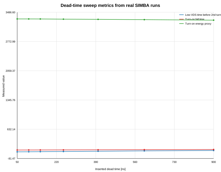
The 1D sweep remains useful because it shows the direction of change on one operating point. The low-VDS interval before the second turn-on rises from about 80.7 ns at 50 ns dead time to 113.5 ns at 900 ns dead time. Over the same range, the measured VDS fall time increases moderately, while the integrated VDS·ID turn-on metric changes only slightly.
That is an honest result, but by itself it is not the most interesting part of the article. The real design insight appears when current is added as a second sweep dimension. The 1D study shows the method. The 2D study shows why the method matters.
4. What the waveforms actually look like
4b. Adding current as a second sweep dimension
The first sweep answered a narrow question: what changes with dead time on one operating point. To make the study more useful, I extended it with a second parameter: the current level at the second turn-on.
I kept the same official SIMBA Double_Pulse_test design and changed the inductance to obtain higher current during the second pulse. That produced four current regions, approximately:
- 8.2 A
- 14.8 A
- 28.6 A
- 50.7 A
This changes the article substantially. It is no longer only a dead-time sweep. It becomes a dead-time-versus-current exploration.
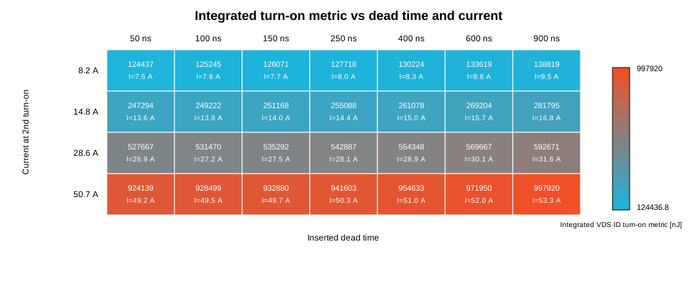
Figure 4 shows that the integrated VDS·ID turn-on metric is far more sensitive to current level than to dead time alone. The metric moves from about 124 µJ near 8 A to almost 998 µJ near 51 A. That immediately gives the article a more realistic power-device perspective.
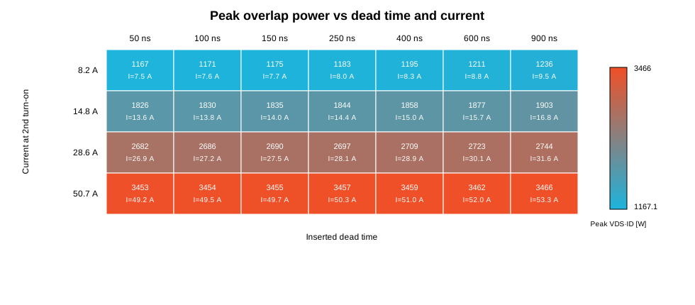
Figure 5 shows the same pattern for peak overlap power. The event rises from roughly 1.17 kW to 3.47 kW across the explored current range. In comparison, dead time still matters, but it is clearly the secondary parameter here.
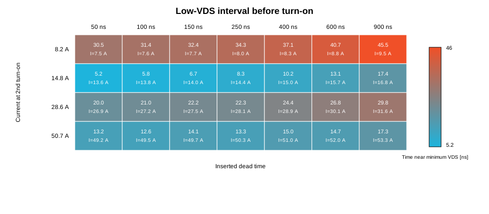
Figure 6 is especially useful for interpretation. At moderate current, increasing dead time increases the low-VDS interval before the next turn-on. But once current rises, that interval becomes much smaller and more sensitive to the commutation conditions. This is the practical reason not to carry one fixed dead-time number from one operating point to another.
5. What an engineer should take from this
Three practical conclusions come out of this sweep.
5.1 Dead time should be swept, not copied
The trend is measurable even over a sub-microsecond range. If a parameter changes the waveforms measurably, it deserves a sweep, not a fixed default value.
5.2 The right metric is not only dead time itself
A dead-time value is not informative by itself. What matters is the event it creates:
- is the node already near low VDS before turn-on?
- what is the remaining overlap power?
- how sensitive is that result to current, bus voltage, or gate resistance?
At a more aggressive operating point, the same workflow should be extended toward metrics that SiC designers immediately recognise, such as:
- diode-conduction interval before the next turn-on
- reverse-current interval
- switching energy extracted over a clearly bounded event window
- margin to low-VDS turn-on or quasi-ZVS behavior
- sensitivity to load current, not dead time alone
5.3 One operating point is not enough
This article is intentionally a first step. It demonstrates the methodology on a real SIMBA double-pulse design and a real transient sweep. The next engineering step would be to extend the sweep over:
- current level
- gate resistance
- bus voltage
- external parasitic inductance
Extending the same workflow to a 2D sweep, dead time versus current, makes the conclusion much stronger. That second sweep is now part of the article, which is why the discussion is no longer limited to a single low-current operating point.
6. Reproducing these results
The study relies on the official SIMBA double-pulse example and on transient sweep results generated from that model during this work.
Official SIMBA documentation: - Python examples overview: https://doc.simba.io/python_api/examples/ - Design examples reference: https://doc.simba.io/python_api/generated_doc/Simba.Data.DesignExamples/
Minimal Python starting point:
import aesim.simba as simba

design = simba.DesignExamples.Double_Pulse_test()

# Example parameter changes
# design.Circuit.GetDeviceByName('V_bus').Value = 800.0
# design.Circuit.GetDeviceByName('L').Value = 200e-6
# design.Circuit.GetDeviceByName('Rg').Value = 5.0
# design.Circuit.GetDeviceByName('Pulse').TimeValueMatrix = ...

job = design.TransientAnalysis.NewJob()
job.Run()
for meta in job.GetSignalsMetadata():
    print(meta.Name)
Files produced in this draft workspace:
deadtime_sweep_results.jsoncase_50ns.jsoncase_250ns.jsoncase_900ns.jsonfig1-deadtime-sweep.svgfig2-waveforms-comparison.svgfig3-circuit.svg
7. Limits of this study
This article now shows a real 2D SIMBA exploration, dead time versus current, so its scope is stronger than the first draft. Still, it remains a methodology article, not a universal SiC design rule.
What it demonstrates credibly:
- a real SIMBA double-pulse workflow
- a real dead-time sweep on an official example
- a real extension toward higher-current operating points
- waveform-based interpretation from transient simulations executed during this work
What it still does not claim:
- a universal dead-time rule valid for every SiC half-bridge
- a vendor-specific switching-loss benchmark
- a formal reverse-recovery or ZVS proof
8. Figures
Figure 3. SIMBA double-pulse circuit used as the study base

References
- Mohan, N., Undeland, T. M., Robbins, W. P. Power Electronics: Converters, Applications, and Design
- Erickson, R. W., Maksimovic, D. Fundamentals of Power Electronics
- Buso, S., Mattavelli, P. Digital Control in Power Electronics
- SIMBA documentation, Python examples overview: https://doc.simba.io/python_api/examples/
- SIMBA documentation,
Simba.Data.DesignExamples: https://doc.simba.io/python_api/generated_doc/Simba.Data.DesignExamples/ - Application notes from Wolfspeed, Infineon, and ROHM on SiC double-pulse testing, dead-time selection, and switching-energy interpretation
About the Author
Sophia is a power electronics specialist at Powersys, focused on converter modeling, simulation workflows, and technical content built from real SIMBA studies.
Autonomous transparency: every numerical result and every waveform discussed in this article comes from a real SIMBA simulation executed during this task, based on the official Double_Pulse_test design example. No synthetic waveform or fabricated result was used.


