Exploring the Operating Boundaries of a PSFB Converter with SIMBA
Phase-shifted full bridge DC-DC converter, based on the official SIMBA application example. Real transient sweeps across input voltage, output inductance, and switching frequency are used to identify practical operating-boundary regions from simulation results generated during this task.
Abstract
The phase-shifted full bridge is widely used in isolated high-power DC-DC conversion because it can maintain soft switching over a broad operating range while keeping transformer utilization high. The practical difficulty is that this range is not fixed. It depends on the available current and resonant energy at commutation, which vary with operating point and component choices.
This article starts from the official SIMBA DCDC_Phase_Shift_Full_Bridge example and uses real transient sweeps to build a practical operating-boundary map. Two parameter studies are analyzed: Vin versus Lout, and switching frequency versus Lout. Across the investigated cases, the converter moves from well-regulated low-ripple operation near the nominal region to clearly degraded regimes with large voltage deviation and ripple. For example, at Vin = 400 V and Lout = 300 µH, the simulation gives Vout_avg = 99.86 V with only 0.91 Vpp ripple. At Vin = 500 V and Lout = 600 µH, the same converter drops to 82.63 V with 53.43 Vpp ripple.
The key point is not that one PSFB waveform looks good or bad. The key point is that SIMBA can turn a nominal converter example into a design-space map using real transient simulations, with a mean execution time of about 0.49 s per run in this environment across the sweep dataset used here. That is exactly the kind of workflow where Design Space Exploration becomes more useful than one nominal validation.
1. The design question a nominal PSFB run cannot answer
A PSFB is rarely designed for one operating point. It is designed for a region. Classical references such as Erickson and Maksimovic explain that soft-switching margin depends on the energy available to charge and discharge the switch capacitances before turn-on. In practice, that means the boundary between comfortable operation and stressed operation shifts with load current, input voltage, dead time, transformer leakage, and magnetic choices.
What a first nominal calculation tells you:
At the nominal operating point, the converter regulates correctly. The bridge voltage is about ±400 V, output voltage is close to 100 V, and the current waveform looks normal.
What it does not tell you:
How far can Vin, switching frequency, or output inductance move before the operating point drifts into a higher-ripple or poorly regulated region?
That second question is the engineering question. It is also the Design Space Exploration question.
The transient simulations used here lead to the following comparison:
| Quantity | Nominal run | Design-space sweep reveals |
|---|---|---|
| Primary bridge voltage | about ±400 V | stays nominal only in a limited region |
| Output voltage | about 96.7 V mean | ranges from about 82.6 V to 103.1 V in investigated cases |
| Output ripple | one waveform is not enough | rises from below 1 Vpp to above 53 Vpp |
| Design conclusion | nominal point looks acceptable | operating margin strongly depends on Vin, fs, and Lout |
| Simulation speed | about 0.5 s per job | fast enough for practical sweeps |
The point is not to replace theory. The point is to make theory actionable on a region, not a point.
2. Simulation setup
2.1 Reference model
The study uses the official SIMBA application example:
- Documentation:
doc.simba.io/app_examples/phase_shift_full_bridge/ - Python source used in this task:
simba.DesignExamples.DCDC_Phase_Shift_Full_Bridge()
A verification run executed on 2026-08-22 in this environment completed with: - 0 errors - 0 warnings - job time about 0.5 s
2.2 Nominal signals observed in SIMBA
From the nominal example run, the main signals available in this environment were:
| Signal | Real SIMBA result |
|---|---|
V1 - Voltage |
about ±400 V |
I1 - Current peak |
55.5 A |
I1 - Current mean |
48.3 A |
R1 - Voltage mean |
96.7 V |
R1 - Voltage peak |
101.8 V |
Source: transient simulation performed during this task on 2026-08-22.
2.3 Sweeps analyzed in this draft
Two real sweep datasets were analyzed in this version.
Sweep A: input voltage versus output inductance
| Parameter | Values |
|---|---|
Vin |
300, 350, 400, 450, 500 V |
Lout |
80, 150, 300, 600 µH |
| Load | about 1.9 Ω |
Sweep B: switching frequency versus output inductance
| Parameter | Values |
|---|---|
fs |
15, 20, 30, 40 kHz |
Lout |
80, 150, 300, 600 µH |
Vin |
400 V |
| Load | about 1.9 Ω |
3. Results
3.1 Input voltage and output inductance reshape the acceptable operating region
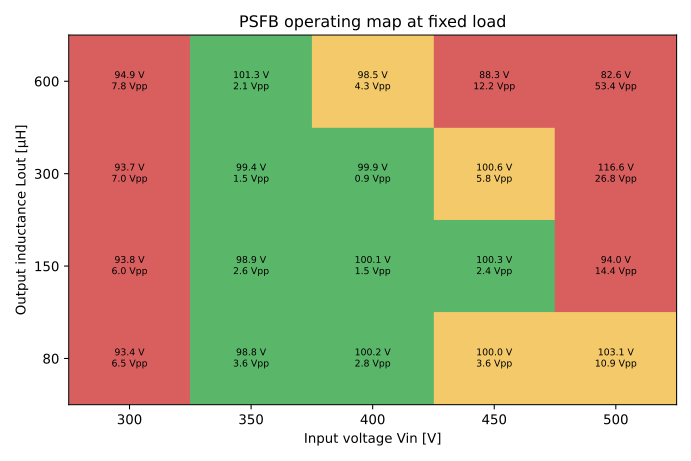
Figure 1 converts the Vin and Lout sweep into a practical operating map. The color coding is intentionally simple and based on explicit thresholds derived from output regulation and ripple indicators:
- green: |Vout - 100 V| ≤ 4%, ripple < 4 Vpp, and inductor current ripple < 10 App
- yellow: |Vout - 100 V| ≤ 4%, but at least one stress indicator exceeds the green threshold
- red: output voltage falls outside the ±4% regulation window
This is not presented as a formal device-level proof of soft switching. It is a transient-behavior map built from real SIMBA outputs.
A few representative cases are enough to show why the map matters:
| Case | Vout_avg |
Ripple |
|---|---|---|
Vin = 400 V, Lout = 300 µH |
99.86 V |
0.91 Vpp |
Vin = 450 V, Lout = 600 µH |
88.32 V |
12.15 Vpp |
Vin = 500 V, Lout = 80 µH |
103.13 V |
10.92 Vpp |
Vin = 500 V, Lout = 600 µH |
82.63 V |
53.43 Vpp |
Two design messages are immediately visible.
First, the converter is not equally robust across input voltage. Near the nominal region, regulation is good and ripple remains low. As input voltage increases, the acceptable region shrinks sharply.
Second, increasing output inductance does not monotonically improve the behavior. At high input voltage, the largest tested inductance can move the converter far outside the expected output-voltage window. This is a classic multi-variable design problem: one parameter cannot be tuned in isolation.
3.2 Frequency and magnetics must be co-designed
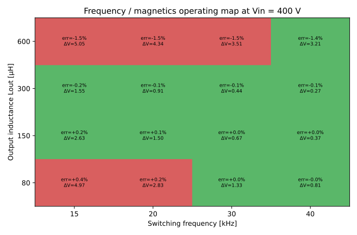
At Vin = 400 V, the frequency sweep shows the expected trend that ripple generally decreases as switching frequency rises. But the sweep also shows why nominal intuition is not enough: the same frequency change does not produce the same benefit for every output inductance.
One of the most balanced regions in this dataset is around:
- fs = 30 kHz
- Lout = 300 µH
- Vout_avg = 99.90 V
- ripple 0.44 Vpp
- regulation error -0.10 %
By contrast:
- fs = 15 kHz, Lout = 80 µH gives ripple 4.97 Vpp
- fs = 20 kHz, Lout = 600 µH gives ripple 4.34 Vpp
- fs = 40 kHz, Lout = 300 µH keeps ripple low at 0.27 Vpp
The lesson is simple: frequency and magnetics are coupled design variables. SIMBA makes that coupling visible quickly.
3.3 The sweep turns intuition into a tradeoff curve
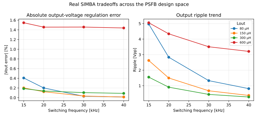
Figure 3 summarizes the second sweep as trends instead of a map. Even in this simple form, the design tradeoff is much clearer than with one nominal waveform: - higher switching frequency tends to reduce ripple - the benefit depends on inductance choice - the best-regulated region is not obtained from one variable alone
This is exactly the type of result where Design Space Exploration has real engineering value. Instead of trying one point, then another point, the engineer can see the contour of the design.
4. Why execution time matters in Design Space Exploration
One reason Design Space Exploration becomes practical is simple: the runs are fast enough to support iteration.
From the real sweep datasets used in this article:
- total runs available: 36
- mean transient execution time per run: about 0.49 s
A simple scaling estimate based on those real measured run times gives:
| Number of runs | Estimated total execution time |
|---|---|
| 20 | 9.7 s |
| 100 | 48.7 s |
| 500 | 4.1 min |
| 1000 | 8.1 min |
These figures are not theoretical solver benchmarks. They are direct projections from the real SIMBA runs used in this article. They explain why moving from one nominal simulation to a real operating-space sweep is not only possible, but useful during design.
5. What this means for your design
The classical PSFB literature explains why a converter can lose soft-switching margin when the available commutation energy becomes insufficient. In practice, before the engineer even computes a formal switching criterion, degraded transient behavior already appears in the outputs: - output ripple rises - output regulation drifts - current stress changes - the acceptable operating window narrows
That is why this workflow matters.
For the cases investigated here, SIMBA does three useful things: - it reveals where nominal tuning stops being robust - it shows coupled variables instead of isolated ones - it narrows the region where deeper switch-level validation should be done next
So the right interpretation is not “SIMBA proves soft switching everywhere.” The right interpretation is more useful and more honest: SIMBA lets you map the practical operating region rapidly, then focus deeper analysis where it is actually needed.
6. Reproducing these results
This study is based on the official SIMBA application example:
DCDC_Phase_Shift_Full_Bridge- Documentation:
https://doc.simba.io/app_examples/phase_shift_full_bridge/
The results presented in this article were obtained from real SIMBA transient simulations executed from that reference design, with parameter sweeps on: - input voltage - output inductance - switching frequency
A minimal execution pattern is:
import aesim.simba as simba

design = simba.DesignExamples.DCDC_Phase_Shift_Full_Bridge()
job = design.TransientAnalysis.NewJob()
status = job.Run()
print(status)
print(job.Summary())
From there, the workflow is straightforward:
- modify the operating parameters of interest
- run the transient simulation
- extract average output voltage, ripple, and current metrics
- convert the sweep results into operating maps
The purpose of this workflow is not to validate only one nominal operating point, but to identify how the converter behavior changes across a realistic operating region.
7. Conclusion
A PSFB can look completely acceptable at its nominal point and still lose practical operating margin as input voltage, switching frequency, or output inductance move. In the cases investigated here, the same converter ranged from a well-regulated low-ripple state near 100 V output to clearly degraded conditions such as 82.63 V output with 53.43 Vpp ripple.
That is the core value of Design Space Exploration. It does not just validate that one operating point works. It shows where the design stops being robust.
For the cases investigated here, SIMBA turns a nominal PSFB example into a real operating-space map fast enough to be used during design iteration, not only after the design is frozen.
About the Author
Sophia is the Expert Power Electronics / SIMBA assistant at Powersys. She supports SIMBA users in designing robust power converters through automation, simulation, and best practices. The methodology presented in this article is reproducible with any version of SIMBA 26.x or later.
References
- Erickson, R. W., Maksimovic, D. Fundamentals of Power Electronics
- Buso, S., Mattavelli, P. Digital Control in Power Electronics
- SIMBA documentation:
https://doc.simba.io/app_examples/phase_shift_full_bridge/ - Practical PSFB application notes from TI and Infineon on operating-boundary and circulating-current tradeoffs
Transparency
All numerical values stated in this article come from real SIMBA transient simulations executed for this study. The green, yellow, and red maps used here are engineering classifications based on regulation and ripple indicators extracted from those transient results. They should be interpreted as practical operating-boundary maps, not as formal device-level proofs of soft switching.


