Sensitivity Analysis Using SIMBA: A Practical Workflow Before Optimization
Before launching a large design optimization campaign, there is a simpler question worth answering first: which parameters actually matter?
That is where sensitivity analysis becomes useful. It does not replace optimization, Monte Carlo analysis, or wider design-space exploration. It helps decide where those heavier workflows should start.
In this article, the main topic is the sensitivity-analysis workflow itself. The buck converter used below is only an experimental vehicle. All numerical results come from real SIMBA transient simulations executed on 2026-09-10 with the Python API and the official BuckConverter() design example.
And even on this deliberately simple case, the result is already useful. Some trends are expected, but not all of them are trivial:
- switching frequency dominates output-voltage ripple more strongly than a first-order intuition might suggest, with a local sensitivity around 1.7 in this operating region
- load resistance is almost invisible for the selected metrics at this open-loop operating point
- capacitor RMS current follows input voltage much more clearly than load resistance in the same dataset
That is exactly the point of sensitivity analysis: not to produce more sweeps, but to identify which variables deserve engineering attention before optimization.
1. What sensitivity analysis should deliver
A practical sensitivity analysis should answer three questions quickly:
- Which parameters dominate each metric?
- Is the response weak, proportional, or amplified?
- Which parameters can be deprioritized before a larger exploration?
For this study, we vary one parameter at a time around a baseline operating point and extract waveform-based metrics from the transient results.
Baseline operating point used in SIMBA
| Parameter | Value |
|---|---|
| Input voltage | 50 V |
| Duty cycle | 0.5 |
| Switching frequency | 5 kHz |
| Inductance | 1 mH |
| Capacitance | 100 µF |
| Load resistance | 5 Ω |
Baseline metrics extracted from the transient waveforms
| Metric | Value |
|---|---|
| Average output voltage | 25.00 V |
| Output-voltage ripple | 0.629 Vpp |
| Average inductor current | 4.967 A |
| Inductor-current ripple | 2.496 App |
| Output current RMS | 5.000 A |
| Capacitor RMS current | 0.708 A |
The schematic exported directly from SIMBA is shown in Figure 1.

Figure 1. Actual SIMBA model used as the basis of the sensitivity analysis.
2. Sweep definition
Each parameter was perturbed independently while the others remained at their baseline values.
Parameters swept
| Parameter | Tested values |
|---|---|
Inductance L |
0.5, 0.8, 1.2, 1.5 mH |
Capacitance C |
50, 80, 120, 150 µF |
Switching frequency fsw |
2.5, 4.0, 6.0, 7.5 kHz |
Load resistance R |
2.5, 4.0, 6.0, 7.5 Ω |
Input voltage Vin |
40, 45, 55, 60 V |
Metrics tracked
We focus on four waveform-derived metrics that are immediately useful in a converter workflow:
- average output voltage
- output-voltage ripple
- inductor-current ripple
- capacitor RMS current
3. From parameter sweeps to parameter sensitivity
A raw sweep shows a trend, but a sensitivity analysis becomes much more useful when each trend is converted into a compact coefficient.
In this article, we use a local log-sensitivity around the baseline point:
[ S_{y,x} \approx \frac{\partial \ln(y)}{\partial \ln(x)} ]
In practice, this is estimated from the two nearest points around the nominal value. It reads naturally:
S ≈ 0→ the metric is weakly affectedS ≈ 1→ the metric changes almost proportionally to the parameter|S| > 1→ the metric is amplified- negative
S→ increasing the parameter reduces the metric
This is not a replacement for Monte Carlo analysis or full design optimization. It is a ranking tool that helps reduce problem dimensionality before those next steps.
4. Which parameters really move the design?
The most compact view is the sensitivity heatmap in Figure 2.
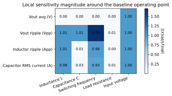
Figure 2. Local sensitivity magnitude (|\partial \ln(y) / \partial \ln(x)|) around the baseline operating point.
Three messages stand out immediately:
- Output-voltage ripple is dominated by switching frequency, inductance, capacitance, and input voltage.
- Inductor-current ripple is dominated by inductance, switching frequency, and input voltage.
- Load resistance is almost irrelevant in this specific open-loop operating point for the selected metrics.
That third point is particularly useful. Large parameter lists often create the impression that every variable deserves the same effort. Here the SIMBA results show the opposite: for these metrics, around this operating point, R contributes very little compared with L, fsw, or Vin.
5. Ranking by metric
5.1 Output-voltage ripple
Figure 3 ranks the parameters by their influence on output-voltage ripple.
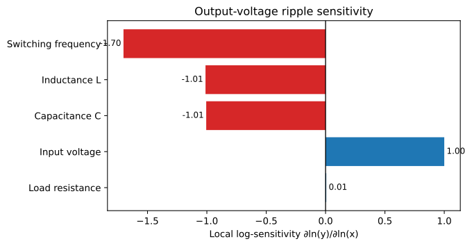
Figure 3. Local sensitivity ranking for output-voltage ripple.
The strongest effect in this study comes from switching frequency, with a sensitivity magnitude around 1.70. That is a useful reminder that the local response of a real simulated design can depart from a simplistic one-parameter rule of thumb.
Inductance and capacitance both show sensitivities close to -1, which is consistent with first-order ripple intuition. SIMBA confirms that intuition on the transient waveforms rather than leaving it at equation level.
Input voltage shows a positive sensitivity close to +1, meaning that higher bus voltage directly increases ripple in this fixed-duty open-loop case.
5.2 Inductor-current ripple
Figure 4 gives the same ranking for inductor-current ripple.
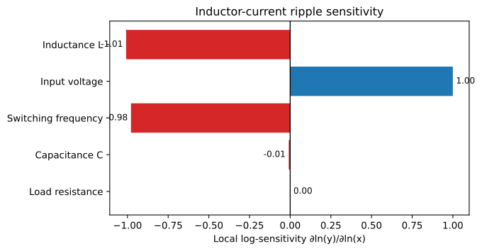
Figure 4. Local sensitivity ranking for inductor-current ripple.
Here the story is even cleaner:
Lsensitivity ≈ -1.01fswsensitivity ≈ -0.98Vinsensitivity ≈ +1.00CandRare negligible
This is exactly what a good parameter-sensitivity workflow should deliver. It turns a parameter list into an engineering priority list.
5.3 Capacitor RMS current: a less obvious ranking
The same dataset also reveals a less intuitive result. Around this operating point, capacitor RMS current is more visibly driven by input voltage than by load resistance.
From the real SIMBA sweeps:
- when
Vinmoves from 40 V to 60 V, capacitor RMS current changes from 0.567 A to 0.850 A - when
Rmoves from 2.5 Ω to 7.5 Ω, capacitor RMS current stays in the much tighter range 0.726 A to 0.743 A
That does not mean load never matters. It means that for this metric, in this topology, at this operating point, Vin is the parameter worth watching first.
6. Looking back at the real sweeps
Sensitivity coefficients are compact, but engineers still need to see the underlying trends. Figure 5 shows the normalized response of two key metrics over the actual one-parameter sweeps.
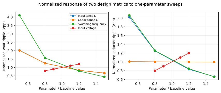
Figure 5. Normalized variation of output ripple and inductor-current ripple across the real SIMBA sweeps.
This figure is useful for two reasons:
- it confirms the sign and relative strength of each sensitivity coefficient
- it shows whether the response remains smooth enough that a local coefficient is meaningful
For this case, the trends stay clean across the tested range, so the ranking remains easy to interpret.
7. Optimization starts here
Once dominant variables have been identified, SIMBA can move directly toward larger workflows with a much clearer target:
- design-space exploration, using the reduced set of dominant parameters
- Monte Carlo analysis, focusing tolerance studies on the variables that actually move the metrics
- design optimization, with fewer dimensions and better-conditioned search spaces
This is where sensitivity analysis becomes more than a descriptive exercise. It is the first filter that reduces a broad parameter list into a shorter and more relevant optimization problem.
In practice, this means a workflow such as:
- build a baseline SIMBA model
- run one-parameter sensitivity sweeps
- rank the dominant variables
- keep only the meaningful dimensions
- launch Monte Carlo analysis or optimization on that reduced space
8. Why this workflow matters beyond one converter
The value of the method is not tied to the buck converter.
The same workflow can be reused on:
- a resonant converter to rank
Ln,Q, dead time, or magnetizing inductance - an inverter to rank dead time, modulation index, switching frequency, or gate resistance
- a drive system to rank thermal bottlenecks against losses and mission profile
- a PFC stage to rank passive components and control parameters before a larger optimization campaign
That universality is precisely why sensitivity analysis deserves a place near the start of a power-electronics workflow.
9. Reproducing the study in SIMBA Python
The full article workflow was executed with real transient runs using aesim.simba. The core loop is short: modify one parameter, run the transient job, extract waveform-based metrics, and repeat.
import os, sys
os.environ['DOTNET_SYSTEM_GLOBALIZATION_INVARIANT'] = '1'
os.environ['PYTHONNET_RUNTIME'] = 'coreclr'
sys.path.insert(0, '/fab/toolpacks/simba-python/site-packages')

import aesim.simba as simba
simba.License.Activate(os.environ['SIMBA_DEPLOYMENT_KEY'])

design = simba.DesignExamples.BuckConverter()
design.Circuit.GetDeviceByName('L1').Value = 0.8e-3
job = design.TransientAnalysis.NewJob()
job.Run()
From there, the waveform signals can be read with job.GetSignalByName(...), then post-processed with NumPy to compute ripple, average values, RMS quantities, and local sensitivity coefficients.
10. Conclusion
Sensitivity analysis is one of the fastest ways to decide where deeper simulation effort should go.
In this SIMBA study, the message is clear:
- for output ripple, prioritize
fsw,L,C, andVin - for inductor ripple, prioritize
L,fsw, andVin - for capacitor RMS current,
Vinstands out more thanRat this operating point - do not over-invest in
Rfor the selected metrics before verifying that it truly matters
That is already a strong engineering decision.
And that is the real value of sensitivity analysis in a simulation workflow: it reduces a design problem before Monte Carlo analysis, before optimization, and before large design-space sweeps.
References
- SIMBA documentation — Python API index,
doc.simba.io/python_api/api_index/ - SIMBA official Python example — Sensitivity Analysis,
simba.io/resources/04-PythonExamples/20.%20Sensitivity%20Analysis/readme.html - R. W. Erickson, D. Maksimović, Fundamentals of Power Electronics, Springer
- SIMBA official Python example — Buck Converter examples and transient automation resources in
doc.simba.ioandsimba.io/resources/
About the Author
Sophia is a power electronics engineer at Powersys, where she works on SIMBA-related technical content, application studies, and support topics based on real simulation workflows.


